Quadrature and Function Approximation
Two new modules, endless fun
Jared Callaham • 21 Sep 2026
Archimedes development has been pretty quiet for the past few months; I’ve been using it for consulting projects, but haven’t had much time for adding new features.
But today’s announcement is a fairly substantial pair of new modules: quadrature and approximation.
These are available as of v0.5.0, and if you’re a current Archimedes user you should be able to upgrade with:
pip install -U archimedes
The quadrature module is for Gaussian-style numerical approximation of weighted integrals:
and approximation is for function representation with linear basis expansions of the form:
Currently supported basis families include:
Orthogonal polynomials, including Legendre, Laguerre, Jacobi, Chebyshev, Hermite, and custom measures.
Piecewise tiling of (most of) the above families (i.e. finite or spectral elements)
Tensor bases for multivariate functions, supporting arbitrary combinations of the above per dimension
Custom bases constructed by constraining or concatenating other bases (e.g. bubble + vertex functions)
These two modules are nicely complementary; quadrature provides the numerical integration used to define inner products between function spaces in approximation, while approximation implements (among other things) the orthogonal polynomial families that Gaussian quadrature is built around.
Those two lines of math are richer than they might appear, especially in terms of their potential applications. To get a sense of this, the rest of the post will walk through a few minimal examples covering PDE solving, trajectory optimization, system identification, and uncertainty quantification - all of which build on the same quadrature and function approximation infrastructure.
Application examples
I’ll be adding several pages to the “tutorials” section of the docs to go into more depth; these are just quick examples to get a feel for how it works and what it can be used for.
The core mechanisms are explained in the “handbook” pages for quadrature and function approximation. To quote the “Function Approximation” page,
There are four key abstractions:
Basis: the definition of the \(\phi(x)\) functions
FunctionSpace: combination of a basis with a domain and associated quadrature rule, together implying an inner product
BasisMatrix: the generalized Vandermonde matrix \(\boldsymbol{\Phi}\) associated with the basis and quadrature rule
Function: A coefficient vector for a particular element of a function space, defining a (piecewise) continuous function in terms of a basis expansion.The four key classes are summarized in the following table:
Math concept
Math notation
Code equivalent
Code convention
Basis functions
\(\{ \phi_i(x) \}_{i=1}^n\)
Basis
phiFunction space
\(\operatorname{span}\{\phi_1, \dots, \phi_n\}\)
FunctionSpace
VGeneralized Vandermonde matrix
\(\boldsymbol{\Phi}_{ij} = \phi_j(x_i)\)
BasisMatrix
PhiFunction
\(f(x) = \sum_{i=1}^n c_i \phi_i(x)\)
Function
f
PDE solving
Linear function approximation underlies many core algorithms for solving partial differential equations, in particular finite element, spectral element, and (pseudo)spectral methods. These mainly differ in terms of (a) which basis they use, (b) how they select quadrature points, (c) how they apply boundary conditions, and (d) how they construct a residual for numerical solution.
The “Hello, world!” of PDE solving is probably the linear Poisson equation
We can construct a “manufactured solution” by choosing some analytic \(u(x)\) and then deriving what \(f(x)\) we’d need to achieve it. A simple one is \(u(x) = \sin(\pi x)\), leading to
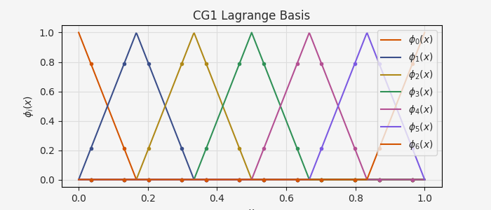
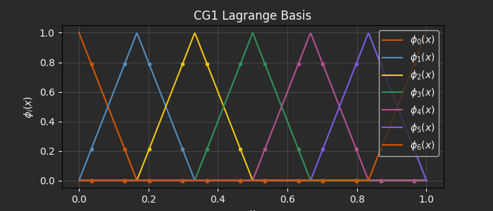
We’ll solve this with a piecewise-linear (CG1) finite element basis:
n_el = 6  # Number of elements
a, b = 0.0, 1.0  # Endpoints
breakpoints = np.linspace(a, b, n_el + 1)

# CG1 Lagrange space
order = 1
V = FunctionSpace.piecewise("lagrange", order, breakpoints)
We’ll solve this in weak form with the Galerkin method. After integrating by parts, the solution \(u(x)\) satisfies the following weak form for any “test function” \(v(x)\) from the same function space:
If we stack all the test functions \(v(x)\) into the \(n_q \times n\) basis matrix \(\boldsymbol{\Phi}\) (for \(n_q\) quadrature points), we can write this as a single linear system:
where \(\mathbf{u}\) and \(\mathbf{f}\) denote the evaluation of \(u(x)\) and \(f(x)\) at the quadrature nodes, \(\mathbf{D}\) is a differentiation matrix, and \(\mathbf{W}\) are the diagonal quadrature weights. Dirichlet BCs are imposed by replacing the test function rows corresponding to the boundaries with the conditions \(u(a) = u_a\) and \(u(b) = u_b\).
This is equivalent to the classical FEA form written in terms of mass and stiffness matrices, but in Archimedes you don’t have to explicitly form mass, stiffness, derivative, or weight matrices:
def u_ex(x):
    return np.sin(np.pi * x)


def f(x):
    return np.pi**2 * np.sin(np.pi * x)


Phi = V.basis_matrix()  # Test functions
dPhi = V.basis_matrix(deriv=1)  # Derivative of test functions
x = Phi.nodes
u0 = V.function()
left, right = V.basis.boundary_dofs()


def res(c):
    u = u0.replace(coefficients=c)

    # Evaluate the residual at the quadrature nodes and project onto the test functions
    lhs = dPhi.T @ u(x, deriv=1)
    rhs = Phi.T @ f(x)
    r = lhs - rhs

    # Dirichlet BCs - set the boundary coefficients directly for Lagrange elements
    r[left] = c[left] - 0.0
    r[right] = c[right] - 0.0
    return r
The weight matrices are applied automatically with matrix multiplication of the transpose Phi.T.
For linear PDEs, this is a single linear solve for the coefficients of \(u(x)\). More generally, this “assembly” step leads to a nonlinear residual, which can be solved with Newton-type root-finding methods:
c0 = u0.coefficients
c_sol = arc.root(res, c0)
u_sol = u0.replace(coefficients=c_sol)

err = np.max(np.abs(u_sol(x_plt) - u_ex(x_plt)))
print(f"max |u_h - u_ex|: {err:.3e}")
max |u_h - u_ex|: 3.287e-02
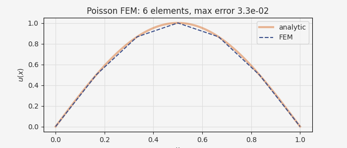
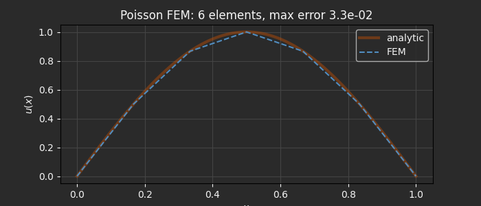
The solution error can easily be reduced by either increasing n_el (\(h\)-refinement) or order (\(p\)-refinement).
This approach can work for nonlinear PDEs as well, and with modifications a similar procedure can be applied to (pseudo)spectral and spectral element methods. One caution, though - the Newton solve here does a direct solve for each linear subsystem. This is fine for 1D and (possibly) small 2D problems on rectangular domains, but for PDE solving work at scale and on real geometries you’ll absolutely still want a specialized library with Krylov solvers, preconditioners, support for unstructured meshes, etc. (Firedrake is my go-to for FEM).
Trajectory optimization
Trajectory optimization is essentially the numerical solution of an optimal control problem: what sequence of inputs should we give a system to get it to minimize some cost or objective function subject to dynamical constraints, endpoint constraints, bounds, and potentially other (e.g. path) constraints. There are many kinds of trajectory optimization and the most common depends on the application domain.
For a quick demo, we’ll look at the classic “block push” (double integrator) problem using a Legendre-Gauss-Lobatto pseudospectral collocation method.
The “block push” problem is
where the dynamics are the double-integrator
Physically, this is a unit mass on a frictionless table, acted on by a force \(u\), with the state \(x\) representing position and velocity. We’d like to move it from rest at position 0 to rest at position 1 with the minimal effort.
Pseudospectral trajectory optimization represents the dynamic state \(x(t)\) and input controls \(u(t)\) with basis expansions:
where \(\ell_i(x)\) are the Lagrange basis functions evaluated at the Gauss-Lobatto quadrature nodes.
This is exactly our linear basis expansion representation, so we can reuse the same function approximation infrastructure, now combined with constrained optimization using minimize.
Collocation is imposed by differentiating the interpolant using the \((n+1) \times (n+1)\) differentiation matrix \(D_{ij} = \ell_j'(t_i)\) and requiring it to match the dynamics at every node:
This is the “defect” constraint. Boundary conditions, path constraints, etc. can simply be concatenated to form the full constraint vector:
t0, tf = 0.0, 1.0
x0, xf = np.array([0.0, 0.0]), np.array([1.0, 0.0])
p = 6  # polynomial degree

quad_rule = arc.quadrature.composite_quad(
    arc.quadrature.gauss_lobatto(p + 1), [-1.0, 1.0]
)
V = FunctionSpace.piecewise(
    "lagrange", p, breakpoints=[t0, tf], nodes="lobatto", quad_rule=quad_rule
)
tp, w = V.quadrature()


def f(x, u):  # noqa: F811
    return np.array([x[1], u[0]], like=x)


def obj(params):
    u_fn = V.function(params["u"])
    return u_fn.dot(u_fn)


def constr(params):
    xp, up = params["x"], params["u"]  # Values at nodes
    x_fn = V.function(xp)

    # State derivative at nodes, from differentiating interpolant
    x_dot = x_fn(tp, deriv=1)

    # Vectorize the dynamics evaluation over the nodes
    x_dot_eval = arc.vmap(f, in_axes=(0, 0))(xp, up)
    defect = x_dot - x_dot_eval

    # Concatenate boundary values
    return np.concatenate([defect, xp[:1] - x0, xp[-1:] - xf]).ravel()


x_guess = x0 + (tp[:, None] - t0) * (xf - x0) / (tf - t0)
init = {"x": x_guess, "u": np.zeros((p + 1, 1))}

res = arc.minimize(obj, x0=init, constr=constr)
sol = res.x
x_opt, u_opt = V.function(sol["x"]), V.function(sol["u"])
The block-push problem has a simple analytic solution:
def x_ex(t):
    return 3 * t**2 - 2 * t**3


def u_ex(t):
    return 6 - 12 * t


t_plt = np.linspace(t0, tf, 1000)
x_plt = x_opt(t_plt)
u_plt = u_opt(t_plt)

print(f"Max absolute error: {max(abs(x_plt[:, 0] - x_ex(t_plt))):.4e}")
Max absolute error: 5.5511e-16
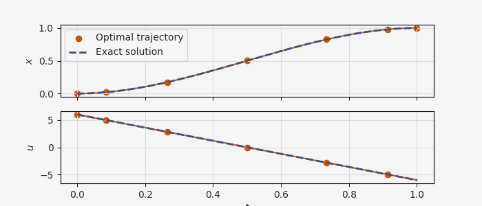
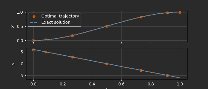
Similar recipes can be used for Hermite-Simpson trajectory optimization, \(hp\)-adaptive pseudospectral collocation on multi-element meshes, and other trajectory optimization formulations.
Eventually the plan is for Archimedes to provide some built-in functionality so you can just pass objective and constraint functions without hand-rolling the discretization, but for now the core quadrature and interpolation/differentiation machinery is there for you to write custom algorithms.
And of course, this is all compatible with the codegen system, so you can either deploy the optimized state/control functions and interpolate them online in a feedforward/feedback scheme, or re-solve the optimal control problem online for a model-predictive control scheme. (Although note that CasADi only supports codegen for certain NLP solvers: SQP but not IPOPT).
System identification
One less obvious place where flexible function approximation can be useful is in gray-box system identification.
The “gray-box” designation here basically means “partially known physics”, and we fill in the gaps with “black box” components.
The approximation module can supply black box components ranging from simple linear lookup tables to B-splines and orthogonal polynomials.
As a simple example, here’s some data generated by simulating a spring-mass system with a complex nonlinear friction law combining Coulomb, Stribeck, and viscous friction. This will be the topic of a full upcoming tutorial or post; this is the quick version.
The basic known physics is Newton’s law: for a known external forcing \(u(t)\), the system evolves according to
The free parameters \(m\) and \(k\) can either be measured directly or inferred via standard parameter estimation. If we don’t know the friction function \(F_f(v)\), we can parameterize it with a basis expansion just as before:
The trick, of course, is choosing which basis expansion to use, and which other constraints will result in a physically meaningful approximation. That’s a rabbit hole we won’t go down today, but you’ll see in a moment what happens when we don’t treat those issues carefully enough.
The data comes from a “chirp” response:
df = pd.read_csv("chirp_response.csv")

data = arc.sysid.Timeseries(
    ts=df["t"].values, ys=df[["x"]].values.T, us=df[["u"]].values.T
)
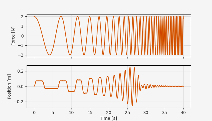
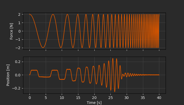
The chirp response shows the characteristic stick-slip pattern at low frequencies, giving way to a more typical resonance peak and then damping.
The following code fits a “gray-box” model to this data; see the parameter estimation tutorial and the Li-ion battery modeling blog post for more background on the prediction error method and system identification. We’ll use a piecewise cubic Hermite polynomial for a smooth but flexible function approximation.
dt = data.ts[1] - data.ts[0]

# Piecewise-cubic Hermite spline
n_el = 2
bkpts = np.linspace(0, 1, n_el + 1)
V = FunctionSpace.piecewise("hermite", 3, bkpts, continuity=1)


@arc.struct
class ModelParameters:
    c: np.ndarray  # Friction coefficients
    k: float  # Spring constant
    m: float  # Mass


# Dynamics model (discretized with RK4)
@arc.discretize(dt=dt, method="rk4", n_steps=1)
def dyn(t, y, u, p):
    x, v = y
    coeffs, k, m = p.c, p.k, p.m

    # Evaluate friction model, imposing symmetry
    friction = V.function(coeffs)
    F = friction(abs(np.atleast_1d(v))).squeeze()
    F = np.where(v >= 0, F, -F)

    # Known physics from Newton's laws
    F_net = -F - k * x + u
    return np.hstack([v, F_net / m])


# Observation model
def obs(t, y, u, p):
    return y[0]  # Observe position


nx, ny = 2, 1  # State and output dimensions

# Set up noise estimates
noise_var = 0.5 * np.var(np.diff(data.ys[0]))
R = noise_var * np.eye(ny)  # Measurement noise
Q = 1e-2 * noise_var * np.eye(nx)  # Process noise

# Extended Kalman Filter for predictions
ekf = arc.observers.ExtendedKalmanFilter(dyn, obs, Q, R)


params_guess = ModelParameters(
    c=np.zeros(V.n_basis),
    k=25.0,
    m=1.0,
)
P0 = 1e-3 * np.eye(nx)  # Initial state covariance estimate
result = arc.sysid.pem(ekf, data, params_guess, x0=np.zeros(2), P0=P0)
Now we can run the model forward to see how well it matches the data. Of course, in a real setting, we’d want to do this against held-out cross-validation data, but this works for a demo. Since we wrote the dynamics function as a discrete RK4 stepper for compatibility with parameter estimation, we’ll just run this as a plain for-loop:
xs_pred = np.zeros((nx, len(data.ts)))
xs_pred[:, 0] = np.zeros(nx)  # Initial state guess
for i in range(1, len(data.ts)):
    t = data.ts[i - 1]
    u = data.us[:, i - 1]
    xs_pred[:, i] = dyn(t, xs_pred[:, i - 1], u, result.p)
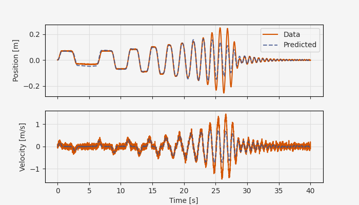
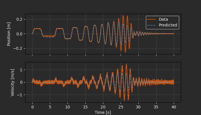
Looks pretty nice! Although one major caveat: this quick-and-dirty parameter estimation run is clearly overfit, with not enough data towards the high-velocity end of the curve. The model is well-behaved for smaller velocities (where it had more training data), but then oscillates wildly and even predicts negative friction at high velocities.
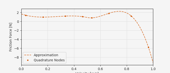
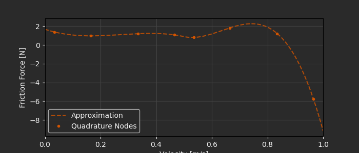
This is (a) why you need cross-validation, and (b) why building in physics-motivated or at least heuristic constraints is crucial for nonlinear system identification.
But again, that’s not the point for today, which is that the approximation module gives you a wide menu of flexible expansion bases that compose cleanly with simulation, optimization, and code generation.
Uncertainty quantification
One other application that might not be immediately obvious is uncertainty quantification. Polynomial chaos in particular relies on function approximations and quadrature in a fundamental way.
The basic idea is to represent a random variable as a function of other random variables using - you guessed it - a linear basis expansion. From Wikipedia directly, for a random variable \(Y\) that depends on other random variables \(X\), the polynomial chaos expansion (PCE) is simply:
The expansion functions are usually orthogonal polynomials that are chosen according to the “Wiener-Askey scheme”. For example, if a variable is normally distributed, you’d use Hermite basis functions (because the weight is Gaussian). For a uniform variable you’d use Legendre (because the weight is uniform), and so on. See the handbook page on quadrature and measures for details.
For a scalar \(X\), the basis functions are the normal flavor we’ve been working with.
For multiple random inputs, you’d typically use a TensorBasis to combine per-input bases constructed based on the input distributions.
The coefficients are determined by L2 projection - literally, evaluating the deterministic function \(f(X)\) at quadrature nodes and summing with quadrature weights. That’s what makes PCE so efficient; you can construct a probabilistic model without randomization or Monte Carlo that converges exponentially quickly in the number of samples. The drawback is that the number of basis functions grows exponentially in dimension, so beyond functions of a few variables you’d need something like Smolyak sparse quadrature, and beyond a few dozen variables… you might be back to Monte Carlo.
Once you have the expansion coefficients, you can trivially compute the mean and variance according to:
Higher moments can also be evaluated as needed, although the formulas are not as simple.
In any case, approximation and quadrature make PCE almost trivial to implement.
Let’s take a simple example with a closed-form solution introduced by the landmark Xiu & Karniadakis (2002) paper that introduced the Wiener-Askey version of PCE that’s dominant today.
The problem is a scalar linear ODE \(\dot{y} = -k y\), with initial condition \(y(0) = 1\) and an uncertain rate constant \(k \sim \mathcal{N}(\mu_k, \sigma_k^2)\). The analytic solution at a fixed time \(t_f\) is
which is itself a random (lognormal) variable with analytic mean and variance
Usually this isn’t available, but we can use it to cross-check the convergence of the numerical approximation.
mu_k = 1.0  # Nominal decay rate [1/s]
sigma_k = 0.3  # Rate-constant uncertainty [1/s]
tf = 3.0  # Evaluation time [s]


def f_decay(k):
    return np.exp(-k * tf)


# Closed-form mean and variance
lam = sigma_k * tf
mu_y_ex = np.exp(-mu_k * tf + 0.5 * lam**2)
var_y_ex = np.exp(-2 * mu_k * tf + lam**2) * (np.exp(lam**2) - 1)

print(f"Exact mean: {mu_y_ex:.6f}")
print(f"Exact std:  {np.sqrt(var_y_ex):.6f}")
Exact mean: 0.074646
Exact std:  0.083387
Constructing a polynomial chaos approximation of \(y\) is simple to implement.
Since \(k\) is Gaussian, we’ll use a (probabilists’) Hermite basis, and since this is a probability distribution we have to add the density=True flag to ensure normalization:
p = 6
V = FunctionSpace.hermite(
    n_basis=p + 1,
    loc=mu_k,
    scale=sigma_k,
    density=True,
)

# The quadrature points are where the projection will sample
x, _w = V.quadrature()
print(f"Number of PCE sample points: {len(x)}")

# Project the forward map onto the Hermite basis
# This is the PCE approximation, then the coefficients give us
# the statistical information.
f_decay_pce = V.project(f_decay)
c = f_decay_pce.coefficients

mu_y_pce = c[0]
var_y_pce = np.sum(c[1:] ** 2)
mu_y_err = abs(mu_y_pce - mu_y_ex)
sigma_y_err = abs(np.sqrt(var_y_pce) - np.sqrt(var_y_ex))
print(f"error on mean: {mu_y_err:.3e}")
print(f"error on std:  {sigma_y_err:.3e}")
Number of PCE sample points: 7
error on mean: 7.982e-10
error on std:  6.965e-06
Pretty good error for a handful of samples! How does this compare to Monte Carlo?
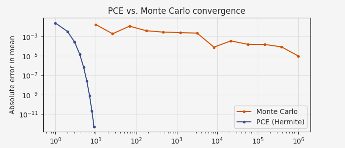
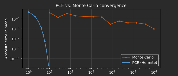
It’s like magic… at least for a univariate function. Again, the number of quadrature points scales exponentially with the dimension of the space \(\sim n^d\) (number of random inputs), so Monte Carlo becomes competitive again after a point.
Still, PCE is useful for cases where function evaluations are expensive, or for applications like optimization under uncertainty where you need tight statistical convergence quickly.
And with the quadrature and approximation modules, you get it almost for free!
A Little History
Now that we’ve seen some of the applications for the quadrature and function approximation infrastructure, I want to zoom out and explain a bit why I’m excited about these new modules, as nerdy as that is.
Archimedes actually began life as a trajectory optimization project I called coco (Collocated Control).
I was trying to write my own version of the legendary GPOPS-ii algorithm based on Rao et al’s papers.
In fact, it actually started in JAX and then moved to Julia before landing on CasADi (but that’s a whole other story).
The original coco code is still on the Archimedes GitHub, and I still think it was a respectable optimal control code.
So after all this time, why hasn’t there been a single trajectory optimization example published in Archimedes?
One reason was just priority; as satisfying as it is to see a trajectory optimization work, there are a lot of great open-source trajectory optimization codes already: acados, Dymos, and PSOPT, to name a few. As a consequence, I thought that a smooth path to hardware for basic control algorithms and real-time simulation could be more impactful than one more trajopt code. As a friend with a lot of experience in automotive controls says, “nobody optimizes anything; in real life it’s all just state machines and lookup tables”.
But more relevant here, the second reason was the coding equivalent of writer’s block. coco included a lot of one-off implementations of things like Gauss-Radau quadrature, barycentric interpolation, and collocation on spectral elements.
My feeling was that these were the tip of some bigger iceberg, but I couldn’t quite figure out what that should be or how to implement it in a useful, modular way.
Eventually, I realized that the unifying theme was the function approximation via linear basis expansion we’ve been discussing throughout this post.
My hope is that implementing these as modular and composable building blocks will support the use cases from the “Applications” section above (including trajectory optimization), but also allow you to build whatever oddball solver or algorithm you want without fully reinventing the numerical wheel.
If you do build something cool with this (and it’s not sensitive or proprietary), feel free to share on the Discussions page! It would be great to see what ends up being useful, painful, or any other feedback.
Read On
There’s a lot of math and code that is barely covered here. For more background on what the new modules do and why, check out the “handbook” pages on quadrature and function approximation.
For more on system identification and how it works in Archimedes, start with the parameter estimation tutorial and Li-ion battery modeling blog post.
More deep-dive posts and tutorials to follow!