Function Approximation¶

This page gives an overview of the infrastructure that Archimedes provides for function approximation with linear basis expansions. All of the methods we will consider approximate methods of the form:

\[f(x) \approx \hat{f}(x) \equiv \sum_{i=1}^n c_i \phi_i(x)\]

With different definitions of the basis, this can encompass a fairly wide variety of numerical methods, from simple lookup tables and power series expansions to complex representations like discontinuous-Galerkin finite element methods and pseudospectral optimal control.

The design of the function approximation system in Archimedes is heavily influenced by other standout packages, most notably chebfun and FEniCS/Firedrake’s Unified Form Language but also shenfun and ApproxFun.jl. What these have in common is that the “function” is a first-class citizen, freeing you to think about what you are modeling instead of bookkeeping nodes, weights, local-to-global maps, and assembly.

So why write a new function approximation module? Archimedes doesn’t claim to beat any of these on their home turf: chebfun and ApproxFun.jl for adaptive, machine-precision work, shenfun for large-scale pseudospectral CFD, and FEniCS/Firedrake for serious FEM work.

What’s new here is composition with the other Archimedes capabilities:

Write a pseudospectral trajectory optimization code using a hierarchical dynamics model and solve the NLP using sparse autodiff
Fit a custom black-box component of a physics-constrained dynamics model using system identification and then deploy a real-time feedforward compensation controller to hardware using C code generation
Approximate continuum mechanics degrees of freedom with a basis expansion, then form the Lagrangian and derive equations of motion using autodiff
Optimize under uncertainty using a differentiable polynomial chaos expansion to model random variables without Monte Carlo

None of these requires working with inflexible pre-rolled APIs that don’t quite do what you want; the system is intended to be composable building blocks in the vein of NumPy/SciPy, giving you the freedom to do whatever you want in the spirit of Archimedes’ “Made for Hackers” philosophy.

This page doesn’t demo any of these itself, but instead provides an introduction to the concepts, abstractions, and interfaces in the module. We’ll start with an overview of the continuous math to establish notation and terminology, then get into the details of the approximation module.

See also:

Quadrature for the Gaussian quadrature module that underpins inner products in approximation

Function Approximation in Brief¶

This is a deep topic, and we will barely scratch the surface here, but the abstract math is not overly complicated and helps to understand the software design. Please forgive any imprecision in the math; this is made by and for engineers.

Function Spaces¶

The core abstraction is a function space, \(\mathcal{V}\) with an inner product \(\langle \cdot, \cdot \rangle_\mathcal{V}\). Specifically, every example we’ll look at uses a weighted inner product on a domain \(\mathcal{D}\), that is:

\[\langle u, v \rangle_\mathcal{V} = \int_\mathcal{D} u(x) ~ v(x) ~ w(x) ~ dx\]

for a weight function \(w(x)\) that depends on the particular function space.

Note that this combination of a domain and weight function is exactly the Measure that underpins orthogonal polynomials and Gaussian quadrature. In fact, the integrals are implemented the quadrature rules supplied by the quadrature module.

That inner product is the key concept; basically everything else is either a consequence of different choices of inner product or of basis functions.

For example, if we work with a basis of functions \(\phi_i(x)\) that are orthogonal with respect to \(w(x)\), then by definition

\[\langle \phi_i, \phi_j \rangle_\mathcal{V} = \|\phi_i(x)\|^2_\mathcal{V} \delta_{ij},\]

where \(\delta_{ij}\) is the Kronecker delta, and

\[\|\phi_i(x)\|^2 \equiv \int_\mathcal{D} \phi_i^2(x) ~ w(x) ~ dx.\]

In this case we can easily extract the expansion coefficients \(a_i\) for any function \(f(x)\):

\[c_i = \frac{\langle \phi_i, f \rangle_\mathcal{V}}{\|\phi_i(x)\|^2}.\]

To make this example more concrete, if \(\mathcal{D}\) is periodic and \(\phi_i(x)\) are Fourier (sine/cosine) functions with \(w(x) \equiv 1\), then this is the familiar spectral projection method taught in undergrad math methods classes.

Galerkin Projection¶

In general the basis functions may not be orthogonal, in which case the coefficient vector \(\mathbf{c}\) for a function can be determined by Galerkin projection, requiring that the approximation residual not lie in the span of the basis vectors. This residual-orthogonality condition is that for any “test” function \(\phi_j(x)\),

\[\langle \phi_j, \hat{f} - f \rangle_\mathcal{V} = 0,\]

where \(\hat{f}(x)\) is again the basis expansion approximation \(\sum_i c_i \phi_i(x)\).

This can be equivalently written as a least-squares problem:

\[\min_\mathbf{c} \bigg| \bigg| \hat{f} - f \bigg| \bigg|_\mathcal{V}^2.\]

Later we will see how this can be implemented with basic matrix multiplications that scale with the number of basis functions.

Petrov-Galerkin Projection¶

As an aside (not critical for what follows), note that it is also possible to draw the test functions from a different basis \(\mathcal{W}\) than the expansion basis (although the weight functions should be the same). This is known as Petrov-Galerkin projection, and the condition is that for any \(\psi \in \mathcal{W}\):

\[\langle \psi_j, \hat{f} - f \rangle_\mathcal{W} = 0.\]

From Continuous to Discrete¶

The inner product is thus a key calculation when working with basis expansions because of its role in finding an L2 projection of an arbitrary function. Of course, the inner product as a (possibly weighted) integral on the domain typically has no useful closed-form solution, so in practice we must resort to numerical quadrature.

Gaussian quadrature approximates the integral with a weighted sum over a fixed set of \(m\) nodes \(\{x_i\}_{i=1}^m\) and weights \(\{w_i\}_{i=1}^m\), chosen so the approximation is exact for the polynomial degrees that appear in the basis:

\[\langle u, v \rangle_\mathcal{V} = \int_\mathcal{D} u(x) \, v(x) \, w(x) \, dx \approx \sum_{i=1}^m w_i \, u(x_i) \, v(x_i).\]

If we construct vectors \(\mathbf{u}\) by sampling the continuous function \(u(x)\) at the quadrature nodes \(\mathbf{x}\), then Gaussian quadrature turns the inner product into a diagonally-weighted dot product of the two vectors \(\mathbf{u}\) and \(\mathbf{v}\). In the event that the basis is polynomial and quadrature rule is chosen to exactly integrate any polynomials that appear in the basis, the quadrature is actually a numerically exact evaluation of the inner product.

This lets us introduce a key construction: the basis matrix (also known as a “generalized Vandermonde matrix”) \(\boldsymbol{\Phi}\), constructed so that the \(j\)-th column is \(\phi_j\) evaluated at the Gaussian quadrature nodes:

\[\boldsymbol{\Phi}_{ij} = \phi_j(x_i), \qquad i = 1, \dots, m, \quad j = 1, \dots, n.\]

Note

The ordinary Vandermonde matrix is the basis matrix for the special case of a monomial basis \(\phi_j(x) = x^{j-1}\)

The basis matrix uses the continuous basis functions sampled at the discrete quadrature nodes, so it is the bridge between the whiteboard theory and the numerical implementation. The basis matrix and the diagonal weight matrix \(\mathbf{W} = \operatorname{diag}(w_1, \dots, w_m)\) allow us to conveniently evaluate a range of operations on basis expansion representations of continuous functions.

For example, the Galerkin projection condition \(\langle \phi_j, \hat{f} - f \rangle_\mathcal{V} = 0\) for every \(j\) can be compactly expressed as the square linear system:

\[\boldsymbol{\Phi}^\top \mathbf{W} \boldsymbol{\Phi} \mathbf{c} = \boldsymbol{\Phi}^\top \mathbf{W} \mathbf{f},\]

where \(f_i \equiv f(x_i)\) is again the continuous function \(f\) sampled at the quadrature points and \(\mathbf{c}\) is the coefficient vector.

Here \(\boldsymbol{\Phi}^\top \mathbf{W} \boldsymbol{\Phi}\) is the Gram (or “mass”) matrix \(\mathbf{M}\) consisting of inner products between two basis functions:

\[M_{ij} = \langle \phi_i, \phi_j \rangle_\mathcal{V},\]

The right-hand side of the projection equation, \(\boldsymbol{\Phi}^\top \mathbf{W} \mathbf{f}\), is the inner product between \(f\) and each element of the basis, which (because of its appearance in linear finite element methods) is sometimes called the load vector \(\mathbf{b}\):

\[b_j = \langle \phi_j, f \rangle_\mathcal{V}.\]

Galerkin projection is then simply the solution to the linear system

\[\mathbf{M} \mathbf{c} = \mathbf{b},\]

which are exactly the normal equations for a weighted least-squares projection.

The `approximation` Module¶

The design of the approximation module follows directly from the theory above.

There are four key abstractions:

Basis: the definition of the \(\phi(x)\) functions
FunctionSpace: combination of a basis with a domain and associated quadrature rule, together implying an inner product
BasisMatrix: the generalized Vandermonde matrix \(\boldsymbol{\Phi}\) associated with the basis and quadrature rule
Function: A coefficient vector for a particular element of a function space, defining a (piecewise) continuous function in terms of a basis expansion.

The four key classes are summarized in the following table:

Math concept	Math notation	Code equivalent	Code convention
Basis functions	\(\{ \phi_i(x) \}_{i=1}^n\)	`Basis`	`phi`
Function space	\(\operatorname{span}\{\phi_1, \dots, \phi_n\}\)	`FunctionSpace`	`V`
Generalized Vandermonde matrix	\(\boldsymbol{\Phi}_{ij} = \phi_j(x_i)\)	`BasisMatrix`	`Phi`
Function	\(f(x) = \sum_{i=1}^n c_i \phi_i(x)\)	`Function`	`f`

Math to Code¶

The operations in From Continuous to Discrete map onto this module in two layers: matrix-level assembly primitives that directly use BasisMatrix, and higher-level Function operations that use them internally.

Assembly Primitives¶

BasisMatrix.T is defined as the adjoint under the weighted inner product, not a plain transpose. This avoids the need to manually track quadrature weights \(W\) in code. So for instance M = Phi.T @ Phi actually computes \(\Phi^\top W \Phi\), and b = Phi.T @ f(x) computes \(\Phi^\top W f(x)\).

Math concept	Math notation	Code
Basis matrix	\([\Phi]_{ij} = \phi_j(x_i)\)	`Phi = space.basis_matrix()`
Derivative basis matrix	\([\Phi']_{ij} = \phi_j'(x_i)\)	`dPhi = space.basis_matrix(deriv=1)`
Mass (Gram) matrix	\(M_{jk} = \langle \phi_j, \phi_k \rangle_\mathcal{V}\)	`Phi.T @ Phi`
Stiffness matrix	\(K_{jk} = \langle \phi_j', \phi_k' \rangle_\mathcal{V}\)	`dPhi.T @ dPhi`
Load vector	\(b_j = \langle \phi_j, f \rangle_\mathcal{V}\)	`Phi.T @ f(x)`

These are commonly used in PDE discretizations (e.g. spectral or finite element methods), but many function approximation applications don’t require directly using these matrix-level operations at all:

`Function` Operations¶

Math concept	Math notation	Code
Inner product	\(\langle u, v \rangle_\mathcal{V} = \int_\mathcal{D} u \, v \, w \, dx\)	`f.dot(g)`
Galerkin projection	\(\min_\mathbf{c} \lVert \hat{f} - f \rVert_\mathcal{V}^2\)	`space.project(f)`
Petrov-Galerkin projection	\(\langle \psi_j, \hat{f} - f \rangle_\mathcal{W} = 0, ~ \psi_j \in \mathcal{W}\)	`space.project(f, test_space=Psi)`
Differentiation	\(f'(x) = \sum_i c_i \phi_i'(x)\)	`f.derivative()`
Antiderivative	\(F(x) = \int_a^x f(t) \, dt\)	`f.antiderivative()`
Definite integral	\(\int_a^b f(x) \, dx\)	`f.integrate()`

Basis Families¶

All of the math and code abstractions above work for any finite-dimensional basis \(\{\phi_i\}_{i=1}^n\). The main choice in function approximation is choosing an appropriate basis for the problem.

The linear-basis-expansion representation is surprisingly broad, including for example:

Monomials (\(1, x, x^2, \dots, x^{n-1}\))
Orthogonal polynomials (Legendre, Hermite, Laguerre, etc.)
Lagrange polynomials (nodal representation)
Fourier series expansions
B-splines
Lookup tables (piecewise linear basis)
Cubic Hermite polynomials
Piecewise finite/spectral element bases
Multivariate tensor product bases

FunctionSpace provides constructors for these common basis families, or you can write your own custom basis and pass it to the general FunctionSpace(basis, domain, reference_quad_rule=...) constructor.

Family	Constructor	Domain	Weight \(w(x)\)	Notes
Legendre	`FunctionSpace.legendre(n_basis, a=-1, b=1)`	\([a, b]\)	\(1\)
Chebyshev	`FunctionSpace.chebyshev(n_basis, a=-1, b=1, second_kind=False)`	\([a, b]\)	\((1-x^2)^{\mp 1/2}\)	`second_kind=True` flips the sign of the exponent
Jacobi	`FunctionSpace.jacobi(alpha, beta, n_basis, a=-1, b=1)`	\([a, b]\)	\((1-x)^\alpha(1+x)^\beta\)
Hermite	`FunctionSpace.hermite(n_basis, loc=0, scale=1, kind="prob")`	\((-\infty, \infty)\)	\(e^{-x^2/2}\) (`"prob"`) or \(e^{-x^2}\) (`"phys"`)
Laguerre	`FunctionSpace.laguerre(n_basis, rate=1, start=0)`	\([\text{start}, \infty)\)	\(e^{-x}\)
Fourier	`FunctionSpace.fourier(n_basis, a=-1, b=1, kind="full")`	periodic \([a, b)\)	\(1\)	`kind="cosine"`/`"sine"` for one-sided trigonometric families; orthonormal by construction
Monomial	`FunctionSpace.monomial(n_basis, a=-1, b=1)`	\([a, b]\)	N/A (not orthogonal)	Power series
Lagrange	`FunctionSpace.piecewise("lagrange", degree, [a, b], nodes="lobatto")`	\([a, b]\)	N/A (not orthogonal)	Nodal (cardinal) basis: coefficients are point values at the chosen node family
Piecewise	`FunctionSpace.piecewise(kind, degree, breakpoints, ...)`	tiled \([a, b]\)	depends on `kind`	Nodal (`kind="lagrange"`) or modal (`kind="legendre"`) local elements, or `kind="hermite"` for \(C^1\) continuity
B-spline	`FunctionSpace.bspline(degree, knots)` / `.clamped_bspline(degree, breakpoints)`	tiled \([a, b]\)	N/A (not orthogonal)	Smooth (\(C^{\text{degree} - 1}\) by default) piecewise polynomials from a knot vector
Tensor product	`FunctionSpace.tensor(*spaces)`	product domain	product of factors’ weights	Multivariate space built from univariate factors

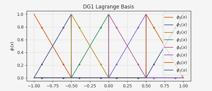
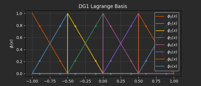
Piecewise is the module’s finite-element basis: kind="lagrange" uses nodal degrees of freedom (point values, the classical FEM element), kind="legendre" uses modal ones, and kind="hermite" adds slope DOFs at each element boundary (needed for 4th-order operators like beam bending). continuity=-1 gives a fully discontinuous (broken) basis.

The easiest way to visualize the basis functions themselves is to construct a function space and then create a Function using a “one-hot” unit basis vector \(\mathbf{e}_i\). For example, here are the leading Legendre basis functions:

n = 5  # Number of basis functions to use
a, b = -1, 1  # Domain bounds

# Basic orthogonal polynomial basis on [-1, 1]
legendre = FunctionSpace.legendre(n, a, b)

x_plt = np.linspace(a, b, 500)
x, _w = legendre.quadrature()

fig, ax = plt.subplots(1, 1, figsize=(7, 3))
for i in range(n):
    # The i-th basis function is the i-th column of the identity matrix
    e_i = np.eye(n)[:, i]
    f_i = legendre.function(e_i)
    ax.plot(x_plt, f_i(x_plt), label=rf"$\phi_{i}(x)$")
    ax.plot(x, f_i(x), ".", color=ax.lines[-1].get_color())


ax.grid()
ax.set_ylabel(r"$\phi_i(x)$")
ax.set_title("Legendre Basis")
ax.legend(loc="upper right")
ax.set_xlabel("$x$")
plt.show()

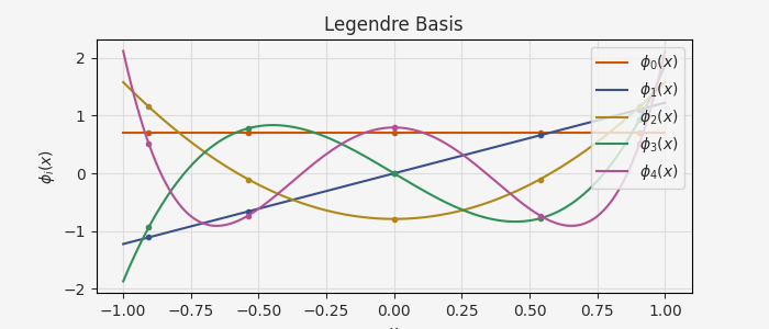
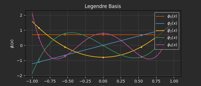
The dots in these plots show the nodes for the associated quadrature rule that will integrate the basis exactly.

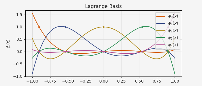
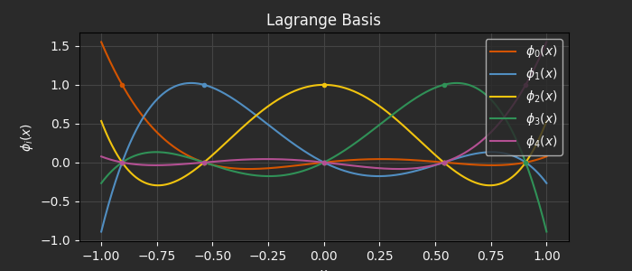
We can use a similar approach to construct a global Lagrange basis. Note that here the basis uses the same nodes as its quadrature rule (Legendre for both), so we can clearly see the defining Lagrange property that the \(i\)-th basis function takes the value 1 at node \(x_i\) and 0 at all other nodes.

We can also use the piecewise constructor to tile the Lagrange basis. The standard finite element basis (CG1, also known as P1) uses Lobatto nodes per element (one node at each basis endpoint), but a Legendre quadrature rule, so now the quadrature nodes are not the same as the Lagrange nodes. Hence, the basis functions are the classical finite element “hat” functions that take on 1 at the element boundaries, but the quadrature nodes are not co-located with the boundaries:

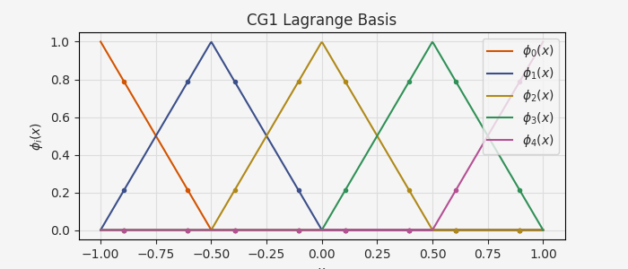
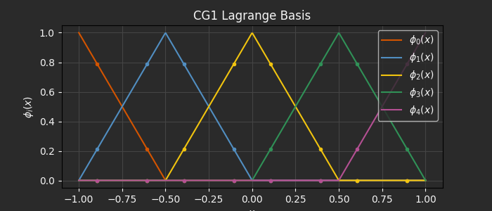
The discontinuous equivalent of the same Lagrange basis (DG1) can be constructed by simply switching to continuity=-1:

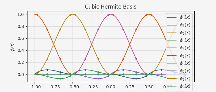
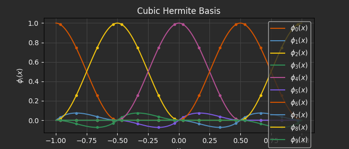
One last example: a piecewise cubic Hermite basis can also be created with the piecewise constructor, and has roughly twice as many basis functions to handle the slope degrees of freedom at element interfaces.

Working with a `Function`¶

As the basis family code snippets show, you typically don’t need to work with the Basis class directly unless you’re constructing a relatively unusual basis. Instead, the FunctionSpace constructors (e.g. FunctionSpace.legendre) will automatically create the Basis for a given domain along with an exact Gaussian quadrature rule.

The same is true of the Function class; a Function is typically created using one of two methods on FunctionSpace:

function_space.function(coefficients=None): directly initializes a Function with known coefficients, defaulting to all zeros if coefficients isn’t passed.
function_space.project(f, quad_rule=None, test_space=None): solve the L2 projection problem for the callable f(x) to establish the coefficients, then return the Function with those coefficients.

L2 projection¶

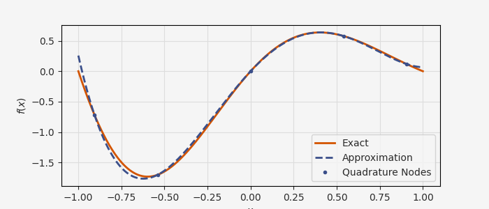
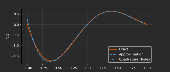
For example, to approximate the function \(e^{-x} \sin \pi x\) using the 4th-order Legendre basis from earlier:

def f(x):
    return np.exp(-x) * np.sin(np.pi * x)


f_approx = legendre.project(f)

Once we’ve created f_approx we can use any of the methods from the Function Operations table:

# Derivative, returned as another Function
df_approx = f_approx.derivative()
print(df_approx(-1.0))

# Compute the definite integral, returning a value
print(f_approx.integrate(0.0, 0.5))

# Compute the anti-derivative (indefinite integral), returning a Function
f_reapprox = df_approx.antiderivative()
print(f_reapprox(-1.0))

-12.555739487273055
0.23115288536913825
1.1102230246251565e-16

Integrals and antiderivatives¶

Note the difference between integrate and antiderivative. The former returns a value (definite integral), while the latter returns a Function (antiderivative, or indefinite integral).

The antiderivative needs to choose a point to start integration from to set the constant of integration. This is specified with the keyword arg boundary and defaults to "left"; on an \((a, b)\) interval:

\[F(x) = \int_a^x f(t) ~ dt\]

The other possibility is boundary="right", which gives:

\[F(x) = \int_b^x f(t) ~ dt = -\int_x^b f(t) ~ dt\]

Note the sign convention here, which is chosen to satisfy the fundamental theorem of calculus with either boundary choice:

for boundary in ("left", "right"):
    F = f_approx.antiderivative(boundary=boundary)
    dF = F.derivative()
    print(f"{boundary} FTOC err: {(dF - f_approx).integrate()}")

left FTOC err: -5.821664841881341e-34
right FTOC err: -5.821664841881341e-34

Although this is numerically exact for the statement that \(F'(x) = f(x)\), the other direction (differentiate first, then integrate) is not exact:

# The leading coefficient (a constant in the Legendre basis) is nonzero
print(df_approx.antiderivative().coefficients - f_approx.coefficients)

[-3.64192230e-01  2.22044605e-16 -6.93889390e-17  0.00000000e+00
  0.00000000e+00]

The reason for this is that even though the underlying \(f(x)\) has \(f(a) = 0\) in this case, the L2 projection does not. But differentiating the basis expansion and then integrating with boundary="left" forces \(f(a) = 0\) rather than choosing the constant to minimize L2 error.

Derivative spaces¶

Note that the derivative method by default returns a Function in the minimal function space needed to exactly represent the derivative. For a first derivative, that’s usually one fewer basis function.

print("n_basis:")
print(f"\tOriginal space:   {f_approx.space.n_basis}")

df_approx = f_approx.derivative()
print(f"\tDerivative space: {df_approx.space.n_basis}")

n_basis:
	Original space:   5
	Derivative space: 4

So by default, the derivative lives in a different space than the original function and the two can’t be directly used together:

try:
    g_approx = f_approx + df_approx
except ValueError as e:
    print(e)

Can only add Functions defined on the same FunctionSpace; project one onto the other's space first, e.g. f + f.space.project(g)

There are two ways around this: either specify the target space on derivative calculation (typically better), or use L2 projection to lift the derivative back to the original space:

# 1. Target space for derivative
df_approx_1 = f_approx.derivative(space=legendre)
print(f_approx.dot(df_approx_1))

# 2. L2 projection back to the original space
df_approx_2 = legendre.project(df_approx)
print(f_approx.dot(df_approx_2))

-0.031016333909177757
-0.031016333909178146

Function Approximation¶

Function Approximation in Brief¶

Function Spaces¶

Galerkin Projection¶

Petrov-Galerkin Projection¶

From Continuous to Discrete¶

The approximation Module¶

Math to Code¶

Assembly Primitives¶

Function Operations¶

Basis Families¶

Working with a Function¶

L2 projection¶

Integrals and antiderivatives¶

Derivative spaces¶

The `approximation` Module¶

`Function` Operations¶

Working with a `Function`¶