Quadrature¶

Quadrature is the name given to a set of algorithms that perform approximate numerical integration of arbitrary functions.

This is a foundational ingredient of a number of higher-level algorithms, including PDE solving, trajectory optimization, and uncertainty quantification. It’s also a different kind of method from time-stepping ODE solvers (odeint, for example). Typical ODE solvers are local, approximating the solution over short interval at a time, whereas quadrature is global, approximating the integrand with an analytically-integrable function on the entire domain at once.

The quadrature module includes support for (mostly) Gaussian quadrature implementations that are compatible with Archimedes’ symbolic tracing, autodiff, and code generation.

This page gives an introduction to numerical quadrature in Archimedes, including the relationship between Gaussian quadrature rules and classical orthogonal polynomials, and how this relationship translates into the concepts of Measure and QuadratureRule.

Quadrature Quickstart¶

Gaussian quadrature approximates a weighted integral with a discrete sum over (generally non-uniform) nodes and weights:

\[\int_a^b f(x) \, w(x) \, dx \approx \sum_{i=1}^n w_i f(x_i),\]

where \(f(x)\) is the function to be integrated, \(w(x)\) is a weight function, and \(\{x_i\}, \{w_i\}\) are the nodes and weights, which are uniquely determined by the family and order of the quadrature rule.

The most common quadrature family, Gauss-Legendre quadrature uses a domain of \([-1, 1]\), with uniform weight \(w(x) = 1\):

\[\int_{-1}^{1} f(x) \, dx \approx \sum_{i=1}^n w_i f(x_i),\]

which can be shifted to an arbitrary (finite) domain \([a, b]\) by rescaling the Gauss-Legendre nodes and weights by:

\[\begin{split}\begin{aligned} x_i &\leftarrow \frac{b-a}{2} x_i + \frac{a+b}{2} \\ w_i &\leftarrow \frac{b-a}{2} w_i \end{aligned}\end{split}\]

Definite integrals on finite domains can be calculated using Gauss-Legendre quadrature with the quadint function:

def f(x):
    return np.exp(x)


a, b = -3, 3  # Integration limits
J_ex = np.exp(b) - np.exp(a)  # Exact integral: e^b - e^a

# 5-point Gauss-Legendre quadrature rule
J_leg = arc.quadrature.quadint(f, a, b, n=5)

print(f"Exact integral:          {J_ex:.6f}")
print(f"Gauss-Legendre integral: {J_leg:.6f}")

Exact integral:          20.035750
Gauss-Legendre integral: 20.035578

Suitably constructed quadrature rules typically converge to an exact result much more quickly than, for instance, uniform trapezoidal integration:

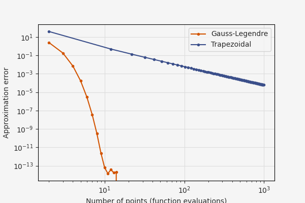
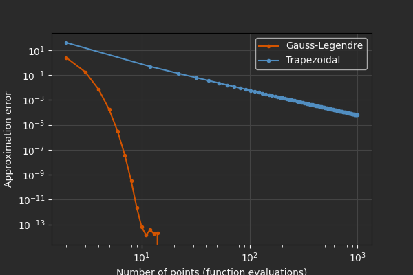
Internally, the integrand evaluation is vectorized; Archimedes-traceable pure functions constructed with NumPy should generally be fine (see Gotchas for more details).

Note that unlike scipy.integrate.quad, this high-level quadint function does not support adaptive integration with an error tolerance, nor does it support infinite or semi-infinite intervals. It is possible to define integrals over infinite or semi-infinite domains using weighted quadrature rules like gauss_laguerre or gauss_hermite, but not through quadint specifically.

Another Quadrature Implementation?¶

NumPy and SciPy already implement the numerical building blocks for Gaussian-style quadrature, and SciPy’s scipy.integrate.quad and relatives is a good choice for evaluating a single integral.

However, for integrals that need to be evaluated inside of simulation or optimization loops, or for any applications that need to support codegen, Archimedes takes advantage of a fundamental split in the quadrature construction. Specifically, on a fixed reference domain (e.g. \([-1, 1]\) for Legendre-based rules), the Gaussian quadrature nodes and weights are static, precomputable data, while the integrand data is symbolic. In fact, internally Archimedes reuses SciPy implementations of node/weight calculations wherever possible.

In other words, the more expensive computation of the rule data can be done once, offline, making the online integral evaluation a simple weighted sum, the equivalent of np.dot(w, f(x)), the cost of which is almost always dominated purely by the integrand evaluation f(x). Domains other than the reference domain can be used with an affine transformation of the nodes and weights, a simple operation for symbolic tracing. This makes it possible for quadrature integrals to compose with the rest of the Archimedes infrastructure, including autodiff, codegen, and hierarchical data structures.

This “traced summation” model precludes adaptive quadrature, because adaptive rules need variable-length vectors for the nodes and weights, which are not supported in Archimedes/CasADi. You could construct a maximum-order-limited adaptive scheme by precomputing nodes and weights for all n < n_max and using control flow primitives, but this isn’t implemented out of the box since it’s not a common use case.

However, Archimedes quadrature does support symbolic evaluation (including limits):

# Differentiating the integral with respect to the limits of integration
def f(x):
    return np.exp(x)


@arc.compile
def integrate_f(a, b):
    return arc.quadrature.quadint(f, a, b, n=5)


dJ_da, dJ_db = arc.grad(integrate_f, argnums=(0, 1))(a, b)

# Analytical derivatives: dJ/da = -e^a, dJ/db = e^b
print(f"Analytical dJ/da: {-np.exp(a):.6f}, dJ/db: {np.exp(b):.6f}")
print(f"Computed dJ/da:   {dJ_da:.6f}, dJ/db: {dJ_db:.6f}")

Analytical dJ/da: -0.049787, dJ/db: 20.085537
Computed dJ/da:   -0.049547, dJ/db: 20.085125

and vector-valued integrands:

# Vector-valued integrands
def f(x):
    return np.array([np.cos(x), np.sin(x)])


a, b = 0, np.pi / 2  # Integration limits
J_vec = arc.quadrature.quadint(f, a, b, n=3)

print("Analytical integral: [1, 1]")
print(f"Computed integral:   {J_vec}")

Analytical integral: [1, 1]
Computed integral:   [1.00000812 1.00000812]

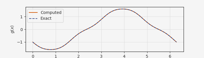
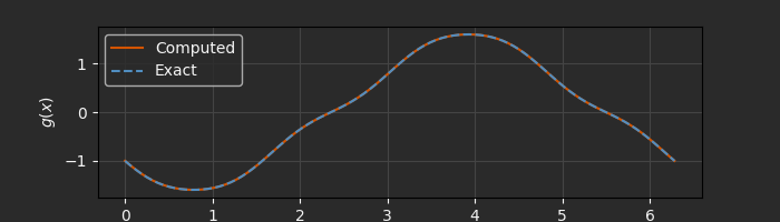
Combining these, you can easily compute derivatives “under the integral sign” using the Leibniz rule:

# https://en.wikipedia.org/wiki/Leibniz_integral_rule#Example_2:_Variable_limits


def f(x):
    return np.cosh(x**2)


def g(x):
    # Variable limits of integration
    a = np.sin(x)
    b = np.cos(x)
    # Compute integral using Gauss-Legendre quadrature
    return arc.quadrature.quadint(f, a, b, n=5)


# Compute g'(x) using automatic differentiation
dg_dx = arc.grad(g)

x = np.linspace(0, 2 * np.pi, 100)
dg = arc.vmap(dg_dx)(x)
dg_ex = -np.cosh(np.cos(x) ** 2) * np.sin(x) - np.cosh(np.sin(x) ** 2) * np.cos(x)

print(f"Error: {np.linalg.norm(dg - dg_ex)}")

Error: 3.2529317769868187e-06

The `quadrature` Module¶

The power of Gaussian quadrature lies in carefully chosen nodes and weights which give highly accurate approximations of integrals of polynomials (and hence arbitrary smooth functions) with relatively few sample points. For instance, the complicated cosh derivative-of-integral above used only five sample points.

The nodes are the roots of classical orthogonal polynomials associated with the weight function (i.e. Legendre polynomials for \(w(x) = 1\) on a finite interval), and the weights are derived from Lagrange interpolation of the nodal data (see the appendix Quadrature and Orthogonal Polynomials below).

Since the nodes and weights on the reference domain can be statically computed, under the hood we use SciPy’s roots_legendre/jacobi/laguerre/hermite functions to do the actual math.

Module Basics¶

There are two abstractions that keep track of the weight function, reference domain, and reference nodes/weights. The first is Measure, which combines a weight function with a reference interval to define families of orthogonal polynomials. The second is QuadratureRule, which stores the nodes, weights, and associated Measure, and which is responsible for domain transformations and performing the weighted sum.

See also:

Approximation for the higher-level function approximation system that relies on quadrature for inner products

`Measure`¶

The Measure class defines an orthogonality measure \(d\mu(x) = w(x) ~ dx\) and an associated domain \(\mathcal{D}\). This \(w(x)\) is the weight function in the quadrature rule, and the quadrature nodes for this rule are the roots of the polynomials that are orthogonal with respect to this measure (see appendix).

The Measure interface is roughly:

class Measure:
    domain: ReferenceDomain  # UnitInterval | HalfLine | RealLine

    # True if closed-form recurrence_coeffs is verified affine-invariant --
    # see "Custom Rules" below
    affine_invariant: bool = False

    # Domain of support D = [a, b]
    @property
    def support(self) -> tuple[float, float]: ...

    # Weight function w(x)
    @abc.abstractmethod
    def weight(self, x: np.ndarray) -> np.ndarray: ...

This might seem obscure, but it is fundamental for designing numerical schemes that aren’t on finite intervals, or for functions with singularities.

Measures are also a useful practical concept for working with probability distributions; in this context a properly-normalized weight function \(w(x)\) is the probability distribution function and the weighted integral is the mean value of \(f(x)\) over that distribution (this is the core of polynomial chaos expansions, for instance).

`QuadratureRule`¶

QuadratureRule is a single class (not a base class or interface) that combines a Measure with associated nodes, weights, and (if a composite/piecewise rule) breakpoints and elements. This is a higher level from Measure because there are different rules that can be constructed on a single Measure. For instance, Gauss-Lobatto and Gauss-Legendre rules both use a uniform measure but different nodes/weights; same for composite (tiled) quadrature rules.

The key parts of QuadratureRule are:

@arc.struct
class QuadratureRule:
    reference: QuadratureReferenceData  # static nodes/weights/measure/breakpoints/elements
    name: str
    params: ReferenceDomain.Parameters | None = None  # the currently-set mapping

    # Nodes/weights on the currently-mapped domain (the reference domain if
    # `map_to` was never called) -- symbolic if the mapping is
    @property
    def nodes(self) -> np.ndarray: ...
    @property
    def weights(self) -> np.ndarray: ...

    # A new rule mapped onto the target domain
    def map_to(self, *params, **kwparams) -> QuadratureRule: ...

    # Approximate the weighted integral of ``f`` over the current mapping
    def integrate(self, f, *, axis=-1, args=None, density=False) -> np.ndarray: ...

    # Quadrature applied to values already sampled at the nodes
    def sum(self, values, *, axis=-1, density=False) -> np.ndarray: ...

Higher-level interface¶

If you’re not constructing exotic custom quadrature rules, you shouldn’t need to interact with either of these classes directly (if you are constructing exotic custom quadrature rules, see below).

Most applications can work with the two high-level interfaces:

The quadint function demonstrated earlier, which takes a callable function and does Gauss-Legendre quadrature on an unweighted finite interval
Convenience constructors for common QuadratureRules like Gauss-Radau, Clenshaw-Curtis, Gauss-Hermite, etc.

We’ve already seen #1 in action; in fact, #1 is just a very thin wrapper around #2 for anyone.

The convenience constructors use snake-case versions of the conventional names of the rules, e.g. Clenshaw-Curtis becomes clenshaw_curtis, and produce a QuadratureRule instance. Available options are:

Classical name	Python function	Weight function \(w(x)\)	Reference interval	Notes
Gauss-Legendre	`gauss_legendre(n, a=None, b=None)`	\(1\)	\([-1, 1]\)	Neither endpoint included
Gauss-Radau	`gauss_radau(n, endpoint="left"\|"right", a=None, b=None)`	\(1\)	\([-1, 1]\)	Fixes one endpoint
Gauss-Lobatto	`gauss_lobatto(n, a=None, b=None)`	\(1\)	\([-1, 1]\)	Fixes both endpoints
Clenshaw-Curtis	`clenshaw_curtis(n, a=None, b=None)`	\(1\)	\([-1, 1]\)	Chebyshev-Lobatto nodes
Trapezoidal	`trapezoidal(n, periodic=False)`	\(1\)	\([-1, 1]\)	Pass `periodic=True` for a Fourier basis
Gauss-Jacobi	`gauss_jacobi(n, alpha, beta, a=None, b=None)`	\((1-x)^\alpha(1+x)^\beta\)	\([-1, 1]\)	Legendre/Chebyshev are special cases
Gauss-Hermite (probabilists’)	`gauss_hermite(n, kind="prob", loc=None, scale=None)`	\(e^{-x^2/2}\)	\((-\infty, \infty)\)	Default `kind`
Gauss-Hermite (physicists’)	`gauss_hermite(n, kind="phys", loc=None, scale=None)`	\(e^{-x^2}\)	\((-\infty, \infty)\)
Gauss-Laguerre	`gauss_laguerre(n, rate=None, start=None)`	\(e^{-x}\)	\([0, \infty)\)

The a/b/rate/start/loc/scale keyword args are sugar for calling .map_to(...) on the freshly-built reference rule – gauss_legendre(n, a, b) is exactly gauss_legendre(n).map_to(a, b).

The trapezoidal rule is slightly different from the others, and comes in two forms selected by the periodic keyword. With the default periodic=False, it’s the usual trapezoidal rule on the closed interval \([-1, 1]\), which is not a Gaussian rule in the sense we have been discussing. With periodic=True, nodes are instead placed on the half-open interval \([-1, 1)\) (since \(-1\) and \(+1\) denote the same point once the domain wraps around), and the rule is exact for trigonometric polynomials \(\cos(k \pi t)\), \(\sin(k \pi t)\) for \(1 \leq k \leq n-1\) – the natural choice of quadrature for a Fourier basis.

Once you have the QuadratureRule object, you can inspect the nodes and weights if you like, or just use its quadrature methods:

QuadratureRule.map_to(**kwparams) returns a new rule with its nodes/weights mapped onto a target domain – **kwparams define the domain and weight transformation, e.g. rule.map_to(a=a, b=b) for Gauss-Legendre (or Radau, Lobatto, Jacobi, Clenshaw-Curtis, or trapezoidal) transforms the domain to \((a, b)\), while rule.map_to(loc=mu, scale=sigma) for Gauss-Hermite on an infinite domain shifts/scales the Gaussian weight function. Called with no arguments, or never called at all, a rule stays on its reference domain.
QuadratureRule.integrate(f) integrates f(x) over whatever domain the rule is currently mapped onto
QuadratureRule.sum(fp) does the same thing but with pre-computed function data on the nodes

The equivalence between the two is literally:

# This:
quad_rule.integrate(f)

# is the same as this:
xp = quad_rule.nodes
fp = f(xp)
quad_rule.sum(fp)

For a one-off integral on a specific domain, the ergonomic pattern is to pass the domain kwargs to the constructor directly rather than mapping a separate rule, e.g. gauss_legendre(n, a, b).integrate(f).

One distinct feature of the Archimedes quadrature interface is that you can optionally pass a density=True keyword arg (to integrate/sum) to directly interpret the weight functions as probability densities. That is, the quadrature result approximates an expectation under the corresponding probability density:

\[\int_{\mathcal{D}} f(x) \, \rho(x) \, dx, \qquad \rho(x) = \frac{1}{\int_{\mathcal{D}} w(x') \, dx'} w(x)\]

For example, we can compute the expectation of \(x^2\) over a normal distribution with mean \(\mu\) and variance \(\sigma^2\) using the probabilists’ Gauss-Hermite quadrature:

def f(x):
    return x**2


mu = 2.0
sigma = 1.5

# kind="prob" is the default
quad_rule = arc.quadrature.gauss_hermite(n=20, loc=mu, scale=sigma)
J = quad_rule.integrate(f, density=True)

print(f"Exact value: {mu**2 + sigma**2:.6f}")
print(f"Quadrature value: {J:.6f}")

Exact value: 6.250000
Quadrature value: 6.250000

This avoids needing to remember to manually divide out the sum of the weights to normalize an expectation integral.

A related difference in Archimedes is doing away with the tradition of naming the physicists’ Hermite polynomials (weight function \(e^{-x^2}\)) plain Hermite and the probabilists’ Hermite polynomials (weight function \(e^{-x^2/2}\)) HermiteNorm - even though it’s not “normalized” in the probability density sense.

Instead, in Archimedes you explicitly choose between probabilists’ and physicists’ Hermite families with the kind = 'prob' | 'phys' keyword arg, as seen above; "prob" is the default, since its weight is (up to normalization) the standard normal density, making loc/scale behave like an ordinary mean/standard deviation.

One subtlety to be aware of: the numeric meaning of scale depends on kind, since it’s paired with the domain rather than the weight. For kind="prob", scale is exactly the standard deviation of the corresponding Gaussian. For kind="phys", whose weight is \(e^{-x^2}\) rather than \(e^{-x^2/2}\), scale is \(\sqrt{2}\) times that standard deviation.

Clenshaw-Curtis¶

Like the periodic trapezoidal rule, Clenshaw-Curtis quadrature is another outlier in this group. It is not a Gaussian quadrature rule associated with a measure with nodes derived from the roots of classical orthogonal polynomials. Instead, the Clenshaw-Curtis nodes are the extrema of the Chebyshev polynomials.

Like Gauss-Lobatto, the Clenshaw-Curtis nodes include the endpoints, but there are a couple of key practical differences that determine which is a better fit.

Theoretically, Gauss-Lobatto has roughly twice the polynomial order of accuracy (although [in practice the gap is much smaller](TODO: REF TREFETHEN))
The Clenshaw-Curtis nodes and weights can be cheaply and accurately computed for much larger \(n\), making it more suitable for applications like large-scale PDE models (e.g. direct numerical simulation of fluid dynamics with pseudospectral methods)
The Chebyshev-Lobatto nodes are nested across doubling \(n\), meaning that the nodes for clenshaw_curtis(n) are all also present in the set of nodes for clenshaw_curtis(2*n)

If these aren’t relevant for your application, in general Gauss-Lobatto is preferable for its accuracy.

Composite Rules¶

Quadrature rules with uniform weight \(w(x) \equiv 1\) can be “tiled” into a composite rule. Mathematically, a composite rule interpolates the data onto a piecewise polynomial that is then integrated exactly with a piecewise quadrature rule.

For example, to construct a quadrature rule for a uniform 10-element domain with third-order Gauss-Legendre quadrature in each element:

nel = 10
p = 3
breakpoints = np.linspace(-1, 1, nel + 1, endpoint=True)
rule = arc.quadrature.composite_quad(
    arc.quadrature.gauss_legendre(n=p + 1), breakpoints=breakpoints
)

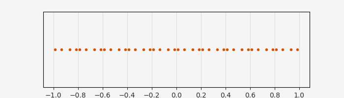
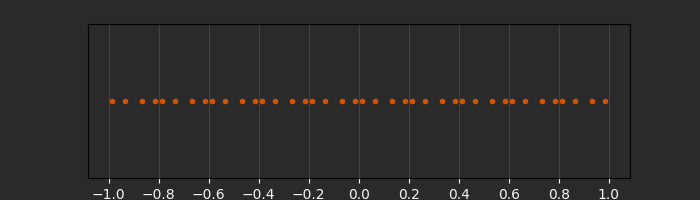
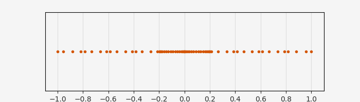
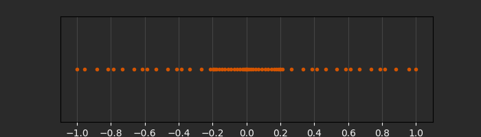
The composite rule does not need to use a uniform degree, nor even a uniform rule. For example, here we add endpoints using left/right Radau rules, and locally refine two interior elements:

el_rules = [arc.quadrature.gauss_legendre(p + 1) for _ in range(nel)]
el_rules[0] = arc.quadrature.gauss_radau(p + 1, "left")
el_rules[-1] = arc.quadrature.gauss_radau(p + 1, "right")
el_rules[nel // 2 - 1] = arc.quadrature.gauss_legendre(4 * (p + 1))
el_rules[nel // 2] = arc.quadrature.gauss_legendre(4 * (p + 1))

rule = arc.quadrature.composite_quad(el_rules, breakpoints=breakpoints)

Tensor Rules¶

A multidimensional product rule can also be constructed via a tensor product of scalar quadrature rules.

For instance, to construct a tenth-order 2D Gauss-Legendre rule:

p = 10
dim_rules = [arc.quadrature.gauss_lobatto(p + 1) for _ in range(2)]
rule = arc.quadrature.tensor_quad(*dim_rules)

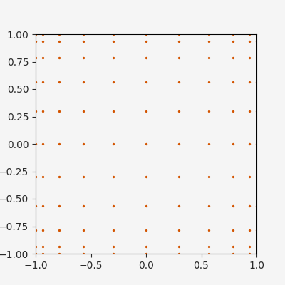
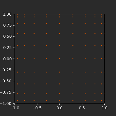
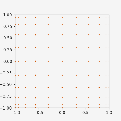
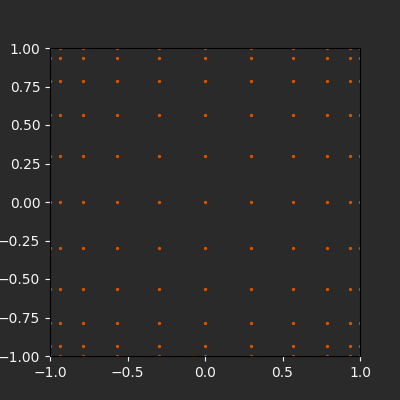
Composite quadrature rules can themselves be expanded with tensor products; copying the non-uniform rule from above:

p = 3
nel = 10
breakpoints = np.linspace(-1, 1, nel+1, endpoint=True)
dim_rules = [
    arc.quadrature.composite_quad(
        arc.quadrature.gauss_legendre(p+1),
        breakpoints=breakpoints
    )
    for _ in range(2)
]
rule = arc.quadrature.tensor_quad(*dim_rules)

Appendix: Quadrature and Orthogonal Polynomials¶

The weight functions, reference domains, and node distributions can seem to be somewhat obscure at first. These arise from a deep connection to classical orthogonal polynomials, and understanding why helps select the right family for an application.

This appendix is fully optional background reading, but may help to explain this interesting connection and why it links together measures, orthogonal polynomials, and optimal quadrature rules - and the implication for numerical schemes like finite elements, pseudospectral methods, etc. that depend on these concepts.

Integration by interpolation¶

The foundational idea of this kind of quadrature is that you approximate the data \(f_i \equiv f(x_i)\) with a polynomial, and then integrate that polynomial exactly. Lagrange polynomials give you a minimum-degree polynomial that exactly interpolates a given set of data; in general \(n\) data points can be exactly interpolated by an \(n-1\)-degree Lagrange polynomial.

In other words, if the function \(f\) happens to be an \(n-1\)-degree polynomial, you can integrate it exactly on any set of \(n\) nodes by constructing a Lagrange interpolating polynomial and integrating it analytically. The weights are the combination of the weight function \(w(x)\) evaluated at the nodes, and the (linear, pre-computable) contribution of the Lagrange polynomial from that node to the integral.

Of course, if \(f\) was a polynomial we could just integrate it analytically anyway, but smooth functions can be accurately approximated with polynomials (and non-smooth functions with piecewise-polynomials), so the exactness of the polynomial degree roughly gives us the accuracy of the method for arbitrary functions.

The genius of Gaussian quadrature is to choose the node positions carefully to get much higher accuracy. For the Gauss-Legendre method, by adding \(n\) additional degrees of freedom to the algebraic problem, we boost the accuracy from \(n-1\) to \(2n - 1\).

Suppose \(f(x)\) is a polynomial of degree \(\leq 2n - 1\), and we will be interpolating at roots \(x_i\). We can construct a polynomial \(q_n(x) \equiv \prod_{i=1}^n (x - x_i)\) and do polynomial long division to decompose into the node polynomial \(q_n(x)\), a quotient \(p(x)\), and the remainder \(r(x)\) (degrees \(n\), \(\leq n-1\), and \(\leq n-1\), respectively):

\[f(x) = q_n(x) p(x) + r(x).\]

We don’t know what \(p(x)\) and \(r(x)\) are here; they’re arbitrary polynomials used to derive the conditions on the selection of roots.

If we apply the quadrature rule \(\sum_{i=1}^n w_i f(x_i)\) to this, by construction \(q_n(x_i) = 0\), so

\[\sum_{i=1}^n w_i f(x_i) = \sum_{i=1}^n w_i r(x_i)\]

If the weights are chosen as above, then since \(r(x)\) has degree \(\leq n - 1\) this integral is exact over \(r\), so

\[\sum_{i=1}^n w_i f(x_i) = \int_a^b w(x) \, r(x) \, dx.\]

In order for this to also equal the weighted integral of \(f(x)\), the additional contribution from \(q_n(x) p(x)\) has to vanish for any polynomial \(p(x)\) with degree \(\leq n - 1\):

\[\int_a^b w(x) \, q_n(x) \, p(x) \, dx = 0.\]

This is exactly the defining property of orthogonal polynomials.

Orthogonal polynomials¶

The important thing for Gaussian quadrature is that given a weight function and a domain, you can derive a family of polynomials such that the \(n\)-th polynomial is orthogonal to all \(n-1\) polynomials in that family with respect to that weight, exactly the property Gauss identifies for optimizing accuracy of the quadrature rule:

\[\int_a^b w(x) \, q_i(x) \, q_j(x) \, dx = 0, \qquad i \neq j\]

Since any \(n-1\)-degree polynomial can be represented by a linear combination of \(q_i(x)\), \(i = 0, 1, \dots, n-1\), the quotient term from polynomial division is guaranteed to vanish.

The upshot is that if we choose the quadrature nodes to be the roots of the appropriate orthogonal polynomial, then we get optimal quadrature accuracy. The “appropriate” polynomial depends on the weight function and the domain, commonly:

Weight \(w(x)\)	Domain	Orthogonal polynomials	Quadrature scheme
\(1\)	\([-1,1]\)	Legendre	Gauss–Legendre
\((1-x)^\alpha(1+x)^\beta\)	\([-1,1]\)	Jacobi	Gauss-Jacobi
\(e^{-x^2}\)	\((-\infty,\infty)\)	Hermite	Gauss–Hermite
\(e^{-x}\)	\([0,\infty)\)	Laguerre	Gauss–Laguerre

The domains (but not their finite-ness) can be adjusted by shifting and scaling the quadrature weights and nodes.

Once the nodes \(x_i\) are determined, the weights are again the combination of the weight function values \(w(x_i)\) and the contribution to the final integral from the associated Lagrange polynomial.

Constrained quadrature schemes¶

The basic Gaussian quadrature methods place \(n\) nodes to be the roots of the \(n\)-th order orthogonal polynomial from the appropriate family. However, these roots don’t inherently include the endpoints of the interval.

Alternatively, we can derive constrained quadrature families that include one or both endpoints; the tradeoff is 1-2 fewer degrees of freedom for the polynomial interpolation and corresponding loss of exactness in polynomial quadrature:

Gauss-Legendre rules: Do not include endpoints - exact to order \(2n - 1\)
Gauss-Radau rules: Include the left or right endpoint (configurable) - exact to order \(2n - 2\)
Gauss-Lobatto rules: Include both endpoints - exact to order \(2n - 3\).

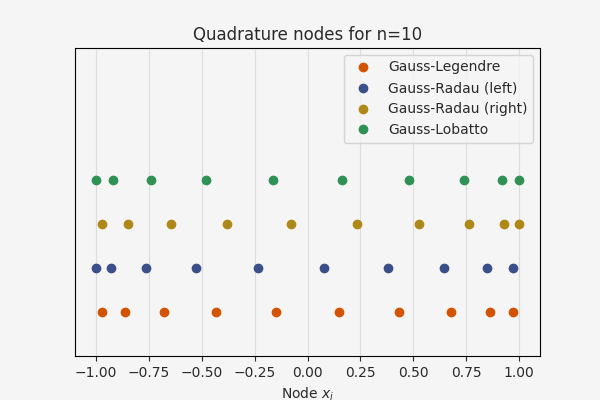
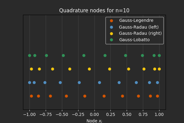
These can be useful for different applications; Gauss-Radau gives useful stability properties for implicit ODE solvers, both Gauss-Radau and Gauss-Lobatto are commonly used in pseudospectral optimal control methods, and Gauss-Lobatto is widely used for high-order spectral element methods.

The schemes themselves are derived similarly to the Gauss-Legendre case, but fixing one of the roots in the polynomial division, e.g. \(q_n(x) = (x - a) q_{n-1}(x)\) for Radau. This amounts to a different weight in the orthogonality requirement and therefore a different member of the orthogonal polynomial family. For Gauss-Radau with an endpoint at \(x = a\) and original weight \(w(x) = 1\), the orthogonality condition becomes:

\[\int_a^b (x - a) \, q_i(x) \, q_j(x) \, dx = 0, \qquad i \neq j\]

That is, the nodes must be placed at the roots of the polynomials that are orthogonal with respect to this inner product with weight \((x - a)\).